Introduction
At this stage, only observations at a single time interval have been retained and data streams (i.e., step lengths, turning angles) have been discretized to perform segmentation on each animal ID. These data are then used as input for the Bayesian segmentation model, which uses a reversible-jump Markov chain Monte Carlo (RJMCMC) algorithm to estimate the breakpoints where values substantially change for the data streams. To facilitate the parallel computation of this model (for each ID), the data must be stored as a list.
library(bayesmove)
library(dplyr)
library(ggplot2)
library(purrr)
library(tidyr)
library(lubridate)
library(furrr)

# Load data
data(tracks.list)

# Check data structure
str(tracks.list)
#> List of 3
#>  $ id1:'data.frame': 4683 obs. of  11 variables:
#>   ..$ id   : chr [1:4683] "id1" "id1" "id1" "id1" ...
#>   ..$ date : POSIXct[1:4683], format: "2020-07-02 12:00:00" "2020-07-02 13:00:00" ...
#>   ..$ x    : num [1:4683] 0 10.6 25.5 31.2 36.2 ...
#>   ..$ y    : num [1:4683] 0 -1.67 -0.61 9.54 19.87 ...
#>   ..$ step : num [1:4683] 10.7 14.97 11.65 11.45 7.24 ...
#>   ..$ angle: num [1:4683] NA 0.227 0.987 0.067 0.032 ...
#>   ..$ dt   : num [1:4683] 3600 3600 3600 3600 3600 3600 3600 3600 3600 3600 ...
#>   ..$ obs  : int [1:4683] 1 2 3 4 5 6 7 8 9 10 ...
#>   ..$ time1: int [1:4683] 1 2 3 4 5 6 7 8 9 10 ...
#>   ..$ SL   : num [1:4683] 5 5 5 5 4 2 5 2 4 5 ...
#>   ..$ TA   : int [1:4683] NA 5 6 5 5 1 5 8 5 4 ...
#>  $ id2:'data.frame': 4697 obs. of  11 variables:
#>   ..$ id   : chr [1:4697] "id2" "id2" "id2" "id2" ...
#>   ..$ date : POSIXct[1:4697], format: "2020-07-02 12:00:00" "2020-07-02 13:00:00" ...
#>   ..$ x    : num [1:4697] 0 -0.00464 0.00375 -0.05953 -0.05953 ...
#>   ..$ y    : num [1:4697] 0 -0.001097 -0.000623 -0.013634 -0.013634 ...
#>   ..$ step : num [1:4697] 0.005 0.008 0.065 0 0.892 ...
#>   ..$ angle: num [1:4697] NA 2.97 -3 2.89 3.11 ...
#>   ..$ dt   : num [1:4697] 3600 3600 3600 3600 3600 3600 3600 3600 3600 3600 ...
#>   ..$ obs  : int [1:4697] 1 2 3 4 5 6 7 8 9 10 ...
#>   ..$ time1: int [1:4697] 1 2 3 4 5 6 7 8 9 10 ...
#>   ..$ SL   : int [1:4697] 1 1 1 1 2 5 3 1 1 1 ...
#>   ..$ TA   : int [1:4697] NA 8 1 8 8 4 8 8 8 6 ...
#>  $ id3:'data.frame': 4716 obs. of  11 variables:
#>   ..$ id   : chr [1:4716] "id3" "id3" "id3" "id3" ...
#>   ..$ date : POSIXct[1:4716], format: "2020-07-02 12:00:00" "2020-07-02 13:00:00" ...
#>   ..$ x    : num [1:4716] 0.00 -6.16e-05 1.34e-01 1.34e-01 -2.60 ...
#>   ..$ y    : num [1:4716] 0.00 -6.58e-05 5.72e-02 5.64e-02 -1.81 ...
#>   ..$ step : num [1:4716] 0 0.145 0.001 3.321 11.272 ...
#>   ..$ angle: num [1:4716] NA 2.728 -2.109 -0.842 0.12 ...
#>   ..$ dt   : num [1:4716] 3600 3600 3600 3600 3600 3600 3600 3600 3600 3600 ...
#>   ..$ obs  : int [1:4716] 1 2 3 4 6 7 8 9 10 11 ...
#>   ..$ time1: int [1:4716] 1 2 3 4 5 6 7 8 9 10 ...
#>   ..$ SL   : int [1:4716] 1 2 1 3 5 1 1 1 1 1 ...
#>   ..$ TA   : int [1:4716] NA 8 2 3 5 7 8 8 1 1 ...
Data for each animal ID are stored separately in each element of the list, where elements include a data frame of the data, including each discretized data stream. Before the model can be run, each of the data frames within the list must only contain a column for the id, as well as the columns that store the discretized data streams.
Run the segmentation model
set.seed(1)

# Define hyperparameter for prior distribution
alpha<- 1

# Set number of iterations for the Gibbs sampler
ngibbs<- 10000

# Set the number of bins used to discretize each data stream
nbins<- c(5,8)

progressr::handlers(progressr::handler_progress(clear = FALSE))
future::plan(multisession, workers = 3)  #run all MCMC chains in parallel
                                         #refer to future::plan() for more details
dat.res<- segment_behavior(data = tracks.list2, ngibbs = ngibbs, nbins = nbins,
                           alpha = alpha)

future::plan(future::sequential)  #return to single core
Now that each of the tracks have been segmented, we need to inspect
the trace-plots for the log marginal likelihood to determine whether the
model converged or not. Additionally, we can inspect a traceplot of the
number of estimated breakpoints per iteration of the RJMCMC for each ID.
Red vertical lines denote the burn-in period for this set of samples,
which is set to 50% of ngibbs by default.
# Trace-plots for the number of breakpoints per ID
traceplot(data = dat.res, type = "nbrks")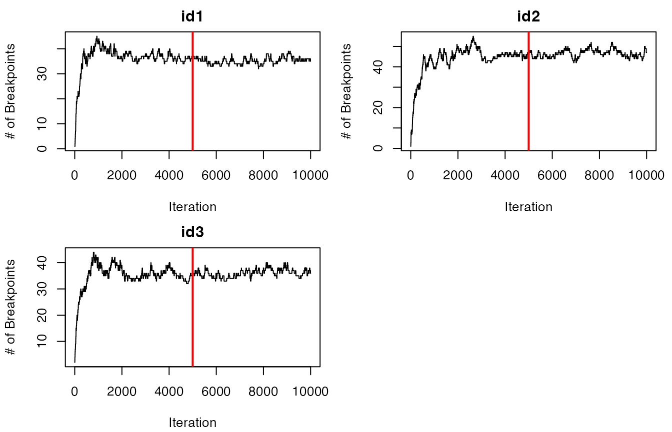
# Trace-plots for the log marginal likelihood (LML) per ID
traceplot(data = dat.res, type = "LML")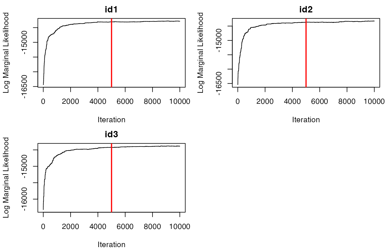
It appears that the models have converged based on the traceplots of
the log marginal likelihoods for all IDs. If this was not the case, the
model would need to be re-run with a greater number of iterations for
ngibbs. It also appears that most IDs likely have 30-40
breakpoints, but the exact number and position of these breakpoints will
be determined by selecting the maximum a posteriori (MAP)
estimate for each animal ID. This is performed as follows:
# Determine MAP for selecting breakpoints
MAP.est<- get_MAP(dat = dat.res$LML, nburn = 5000)
MAP.est
#> [1] 9126 9910 8667

brkpts<- get_breakpts(dat = dat.res$brkpts, MAP.est = MAP.est)

# How many breakpoints estimated per ID?
apply(brkpts[,-1], 1, function(x) length(purrr::discard(x, is.na)))
#> id1 id2 id3
#>  39  49  38
The object MAP.est is storing the iteration at which the
MAP estimate occurs for each ID, whereas brkpts is a data
frame that stores all of the breakpoints per ID. We can plot these
breakpoints over the discretized data streams to inspect how well this
appears to match changes in these values.
Breakpoint visualization
The bayesmove package provides a number of functions to
visualize results from the model, such as traceplot(). The
plot_breakpoints() function provides an easy method to
visualize the breakpoints compared to the data and to determine whether
the number and location of breakpoints appear to be appropriate. The
number and position of breakpoints will depend on a number of factors,
such as the number of observations per ID, the sampling interval of the
biologging device, and the method by which data streams were
discretized. If the breakpoints do not appear to fit the data well, then
the limits used to discretize the data streams likely need to be
modified and the model re-run.
Additionally, there are a number of options to use when visualizing
breakpoints compared to the data streams, such as plotting by
date or by observation (time1). Additionally,
data streams can be visualized on their original scale (continuous) or
as bins. An example is provided here using continuous values for step
lengths and turning angles by observation, but this can be easily
modified.
# Plot breakpoints over the data
plot_breakpoints(data = tracks.list, as_date = FALSE, var_names = c("step","angle"),
                 var_labels = c("Step Length (km)", "Turning Angle (rad)"), brkpts = brkpts)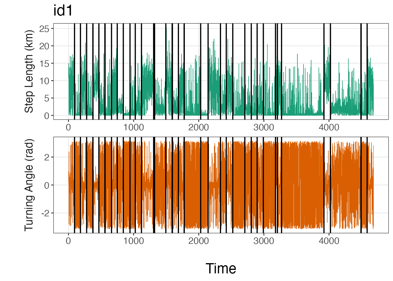
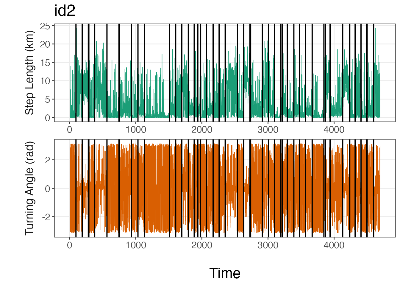
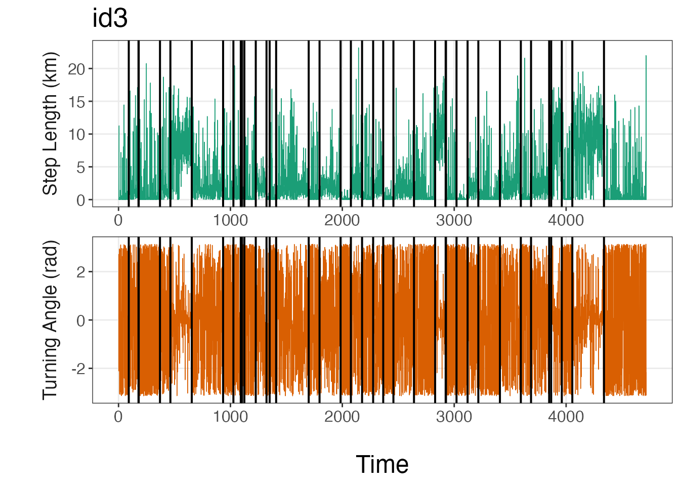
From these lineplots, it appears that the segmentation model
estimated the breakpoints quite well to create relatively homogeneous
units of observations based on SL (step lengths) and
TA (turning angles). If the user would like to plot the
bins instead, they should replace step and
angle with SL and TA,
respectively, as well as the y-axis titles for
var_names.
Now that the MAP estimates of the breakpoints have been identified and we are satisfied with the results, we will use these breakpoints to define track segments of observations for each individual. These segments represent different changes in movement patterns based on the variables that were originally selected.
Assign track segments
# Assign track segments to all observations by ID
tracks.seg<- assign_tseg(dat = tracks.list, brkpts = brkpts)

head(tracks.seg)
#>    id                date        x          y   step  angle   dt obs time1 SL
#> 1 id1 2020-07-02 12:00:00  0.00000  0.0000000 10.695     NA 3600   1     1  5
#> 2 id1 2020-07-02 13:00:00 10.56492 -1.6654990 14.974  0.227 3600   2     2  5
#> 3 id1 2020-07-02 14:00:00 25.50174 -0.6096675 11.653  0.987 3600   3     3  5
#> 4 id1 2020-07-02 15:00:00 31.22014  9.5438464 11.449  0.067 3600   4     4  5
#> 5 id1 2020-07-02 16:00:00 36.15821 19.8737009  7.237  0.032 3600   5     5  4
#> 6 id1 2020-07-02 17:00:00 39.06810 26.4996352  0.119 -2.804 3600   6     6  2
#>   TA tseg
#> 1 NA    1
#> 2  5    1
#> 3  6    1
#> 4  5    1
#> 5  5    1
#> 6  1    1
These segments will then be clustered in the next stage of this Bayesian framework: a mixed-membership Latent Dirichlet Allocation model.